First Happy New Year and best wishes for 2015!
Yes, Data Analytics with R and SQL Server … As Data and Business Intelligence Architects I personally think we just can’t dismiss or push aside the Data Science “landscape”. Hence that’s why I registered and currently more than half way through the Data Science Specialization on Coursera from the Johns Hopkins University. Even though I have been working with R for a while I wanted to get some kind of recognition, attestation for my skills and also just because I can 😉
So the following outlines how to connect to SQL Server with R and briefly highlights some (out of so many more to explore) R functions…
[Required]
Here is what you first need to install to get started:
R
http://www.r-project.org/
RStudio Desktop
http://www.rstudio.com/products/rstudio/
[Optional – but required for this demo!]
For the purpose of this demo I am using the following:
The Adventure Works DW 2014 Database which can be downloaded here https://msftdbprodsamples.codeplex.com/. The demo (and scripts) will also work with the Adventure Works DW 2012 database.
If you decided to use and restore the Adventure Works DW database, you will need to create the following SQL Server View which will serve as our data frame (data table):
CREATE VIEW [dbo].[vw_FactSales]
AS
SELECT	p.EnglishProductName AS 'Product',
        pc.EnglishProductCategoryName AS 'ProductCategory',
        ps.EnglishProductSubcategoryName AS 'ProductSubCategory',
		do.FullDateAlternateKey AS 'DateOrder',
		dd.FullDateAlternateKey AS 'DateDue',
		ds.FullDateAlternateKey AS 'DateShip',
		dc.BirthDate,
		dc.MaritalStatus,
		dc.Gender,
		dc.YearlyIncome,
		dc.TotalChildren,
		dc.NumberChildrenAtHome,
		dc.EnglishEducation AS 'Education',
		dc.EnglishOccupation AS 'Occupation',
		dc.HouseOwnerFlag,
		dc.NumberCarsOwned,
		dc.DateFirstPurchase,
		dc.CommuteDistance,
		g.City,
        g.StateProvinceName AS 'StateProvince',
        g.EnglishCountryRegionName AS 'CountryRegion',
		g.PostalCode,
		pr.EnglishPromotionName AS 'Promotion',
		pr.EnglishPromotionType AS 'PromotionType',
		pr.EnglishPromotionCategory AS 'PromotionCategory',
        cu.CurrencyName AS 'Currency',
		st.SalesTerritoryRegion,
		st.SalesTerritoryCountry,
		st.SalesTerritoryGroup,
		fs.OrderQuantity,
		fs.UnitPrice,
		fs.ExtendedAmount,
		fs.UnitPriceDiscountPct,
		fs.DiscountAmount,
		fs.ProductStandardCost,
		fs.TotalProductCost,
		fs.SalesAmount,
		fs.TaxAmt,
		fs.Freight
FROM    dbo.FactInternetSales fs JOIN
 		dbo.DimProduct p ON fs.ProductKey = p.ProductKey JOIN
        dbo.DimProductSubcategory ps ON p.ProductSubcategoryKey = ps.ProductSubcategoryKey JOIN
        dbo.DimProductCategory pc ON ps.ProductCategoryKey = pc.ProductCategoryKey JOIN
		dbo.DimDate do ON fs.OrderDateKey = do.Datekey JOIN
		dbo.DimDate dd ON fs.DueDateKey = dd.DateKey JOIN
		dbo.DimDate ds ON fs.DueDateKey = ds.DateKey JOIN
		dbo.DimCustomer dc ON fs.CustomerKey = dc.CustomerKey JOIN
		dbo.DimGeography g ON dc.GeographyKey = g.GeographyKey JOIN
		dbo.DimPromotion pr ON fs.PromotionKey = pr.PromotionKey JOIN
        dbo.DimCurrency cu ON fs.CurrencyKey = cu.CurrencyKey JOIN
		dbo.DimSalesTerritory st ON fs.SalesTerritoryKey = st.SalesTerritoryKey
GO
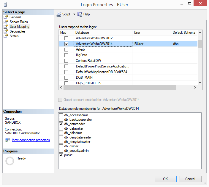
You will also need to create a SQL Server Login named RUser with db_datareader role membership to the Adventure Works DW database
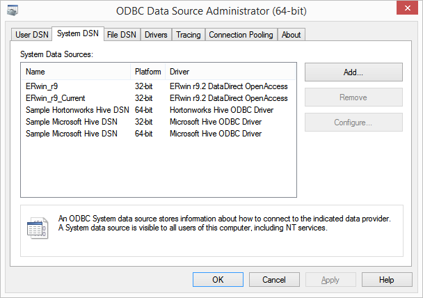
Next we need create a new ODBC System DSN (I opted for 64-bit) click Add
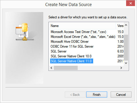
Select SQL Server Native Client 11.0
Name it AdventureWorksDW
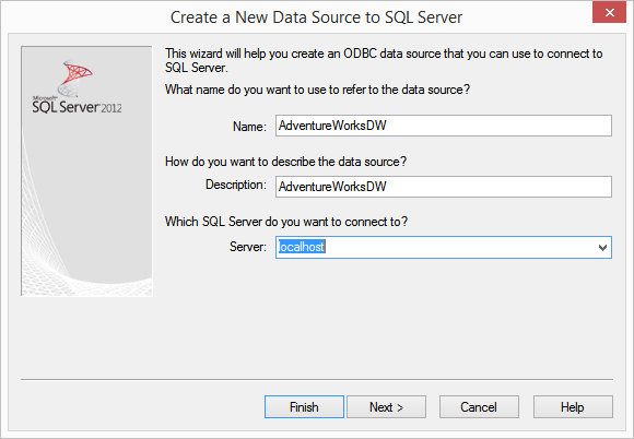
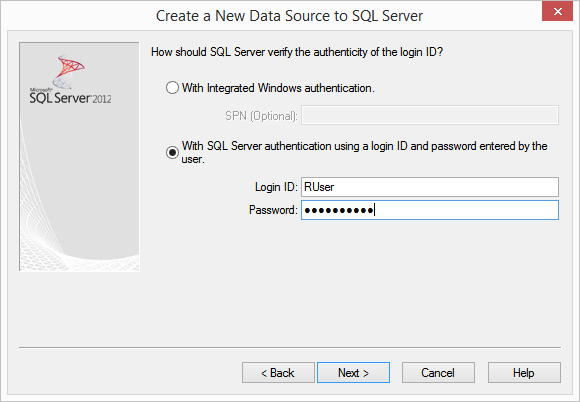
Provide the SQL Server Login information
Change the default database
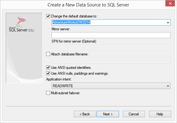
Next
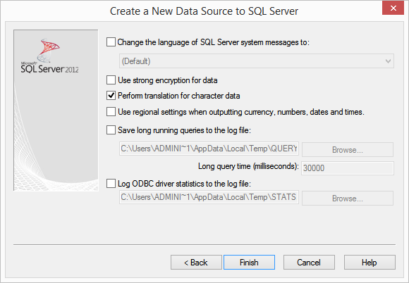
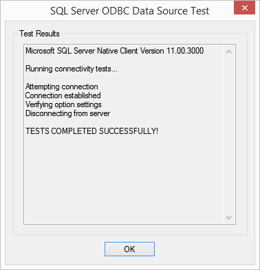
Test connectivity
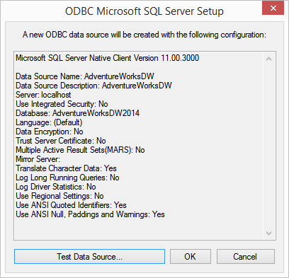
Your done!
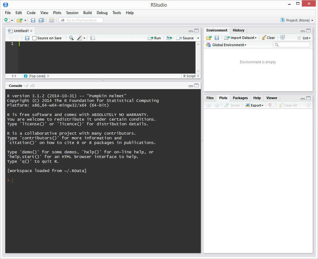
Open RStudio and let’s start exploring. (You will have a different IDE – I am using the ‘Idle Fingers’ theme. To change yours go to Tools – Global Options)
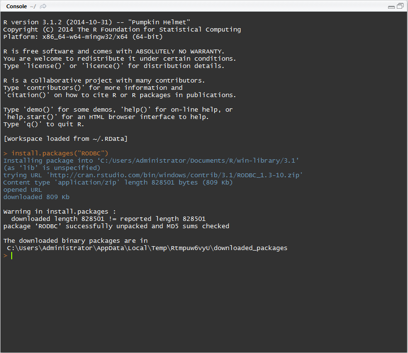
First we need to install a specific package named RODBC which provides ODBC Database Access and will permit us to connect to SQL Server. For more information on the RODBC package follow this link -> http://cran.r-project.org/web/packages/RODBC/index.html
Simply type the following at the prompt in the Console window and press enter.
install.packages("RODBC")
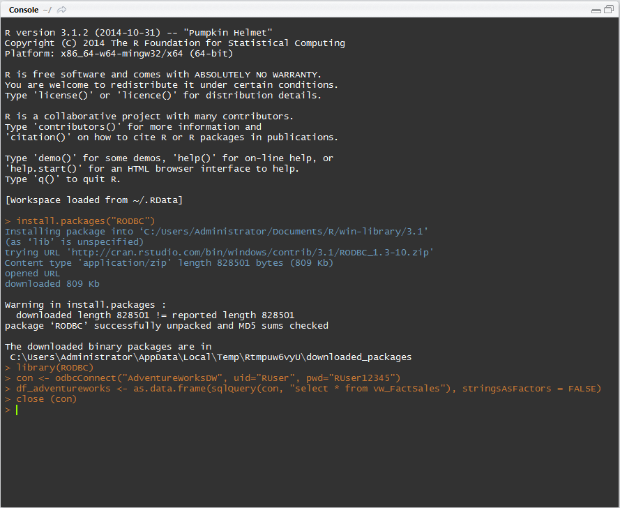
Now we need to load the RODBC package, create a connection “con” to the ODBC DSN “AdventureWorksDW” we created earlier, query the database and put the results into a data frame “df_adventureworks” and close the connection.
library(RODBC)
con <- odbcConnect("AdventureWorksDW", uid="RUser", pwd="RUser12345")
df_adventureworks <- as.data.frame(sqlQuery(con, "select * from vw_FactSales"), stringsAsFactors = FALSE)
close (con)
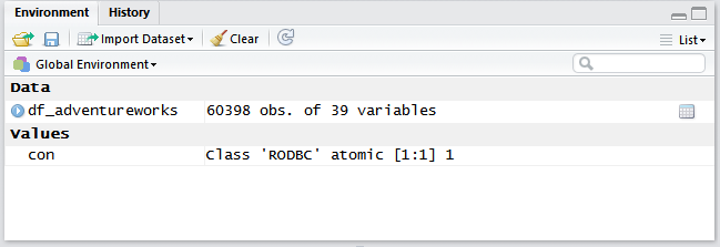
You should see in your Environment window pane the following data frame df_adventureworks with 60398 obs. of 39 variables. Meaning 60398 rows of data with 39 attributes (columns)
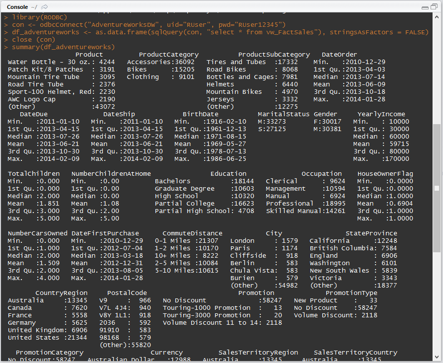
The most useful multipurpose function in R is summary(X) where X can be one of any number of objects, including datasets, variables, and linear models… just to name a few! The summary function has different outputs depending on what kind of object it takes as an argument. Besides being widely applicable, this method is valuable because it often provides exactly what is needed in terms of summary statistics.
Let’s give it a try - type the following command in the Console window and press enter
summary(df_adventureworks)
Take time to look at the generated output (very interesting)
Now let’s look at two other functions colMeans and aggregate
Type the following commands in the Console window and press enter
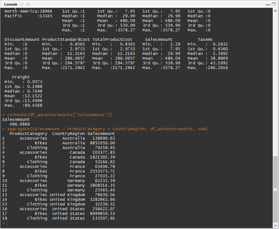
colMeans(df_adventureworks["SalesAmount"])
aggregate(SalesAmount ~ ProductCategory + CountryRegion, data=df_adventureworks, FUN=sum)
colMeans returns the mean for the specified columns, in this case for SalesAmount the mean is 486.0869
aggregate splits the data into subsets, computes summary statistics for each, and returns the result in a convenient form.
Those of you who are familiar with SQL Server will notice that this function “aggregate(SalesAmount ~ ProductCategory + CountryRegion, data=df_adventureworks, FUN=sum)” is somewhat similar to GROUP BY and thus the following T-SQL will return the same results.
SELECT	ProductCategory,
		CountryRegion,
		SUM(SalesAmount) AS 'SalesAmount'
FROM	dbo.vw_FactSales
GROUP BY
		ProductCategory,
		CountryRegion
ORDER BY
		CountryRegion,
		ProductCategory
On to graphics, you can create several basic graph types like density plots, dot plots, bar charts, line charts, pie charts, boxplots and scatter plots in R, I recommend you look at the following link -> http://www.statmethods.net/graphs/index.html to get you started.
But to create advanced graphics in R one needs to install the ggplot2 package.
ggplot2 is an implementation of the grammar of graphics in R. Official documentation can be found at the following link -> http://docs.ggplot2.org/current/
In order to install and use the ggplot2 library, type the following commands in the Console window
install.packages("ggplot2", dependencies = TRUE)
library(ggplot2)
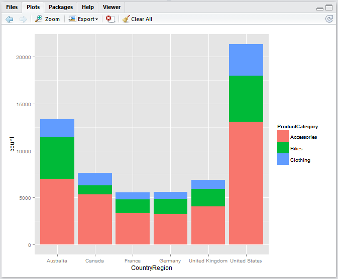
Let’s create a bar plot with the count of sold ProductCategory [Accessories, Bikes, Clothing] by CountryRegion
Type the following command in the console and press enter
ggplot (df_adventureworks, aes(CountryRegion, fill=ProductCategory)) + geom_bar()
The graph will appear in the Plot window and should look similar to the following
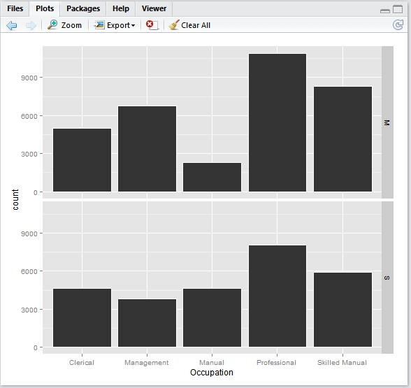
This one will create 2 separate bar plots [MaritalStatus] one for Married and other for Single with count by Occupation
ggplot(df_adventureworks, aes(Occupation) ) + geom_histogram(color = "white") + facet_grid(MaritalStatus ~ .)
Before we wrap up here is the entire R script used for this demo
# Install RODBC package
install.packages("RODBC")

# Load RODBC package
library(RODBC)

# Create connection "con" to SQL Server and database using ODBC DSN
con <- odbcConnect("AdventureWorksDW", uid="RUser", pwd="RUser12345")

# Query the database and put the results into the data frame "df_adventureworks"
df_adventureworks <- as.data.frame(sqlQuery(con, "select * from vw_FactSales"), stringsAsFactors = FALSE)
close (con)

# Return summary statistics about the "df_adventureworks" data frame
summary(df_adventureworks)

# Return the mean for the "SalesAmount" column
colMeans(df_adventureworks["SalesAmount"])

# Return aggregate sum data for "SalesAmount" grouping it by "ProductCategory" and "CountryRegion"
aggregate(SalesAmount ~ ProductCategory + CountryRegion, data=df_adventureworks, FUN=sum)

# Install ggplot2 package and dependencies
install.packages("ggplot2", dependencies = TRUE)

# Load ggplot2 package
library(ggplot2)

# Plot with count (number) of sold "ProductCategory" [Accessories, Bikes, Clothing] by "CountryRegion"
ggplot (df_adventureworks, aes(CountryRegion, fill=ProductCategory)) + geom_bar()

# Plots 2 separate bar plots "MaritalStatus" one for Married and other for Single with count by "Occupation"
ggplot(df_adventureworks, aes(Occupation) ) +  geom_histogram(color = "white") + facet_grid(MaritalStatus ~ .)
To conclude, this is certainly not the best dataset (may want to look at an earlier post for better ones) for performing advanced analytics, but serves great purpose for demonstrating how to connect to SQL Server with R and introduce some basic R functions…
If you are interested to learn more and further explore about R, I strongly recommend you start with the following resources